
ProcessOpt tutorial: SAG Mill PMB and Morrell Power Model
Build a SAG mill model that tracks filling, power and product size - step by step in ProcessOpt
1 Fundamental
A population balance follows the ore inside the mill; the Morrell model turns the charge into power.
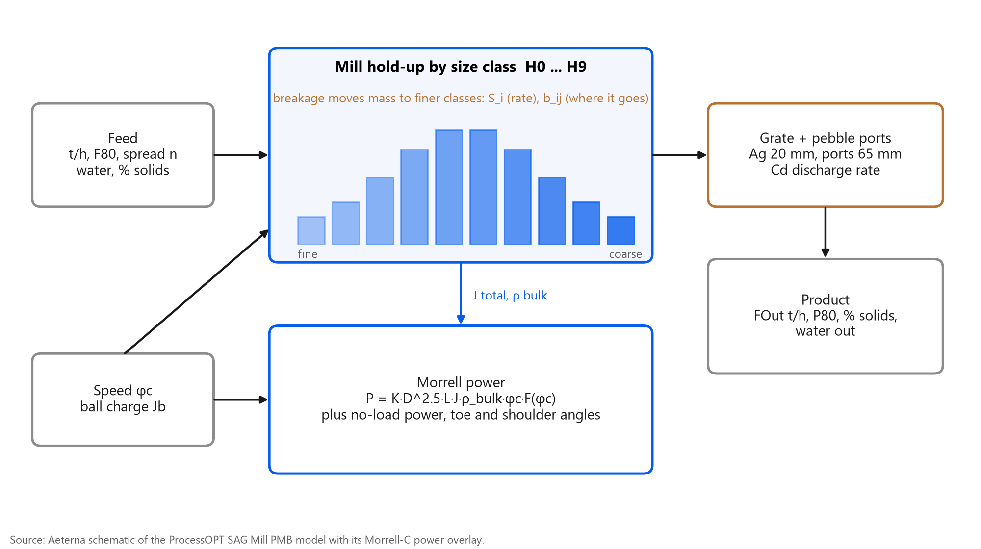
The SAG model tracks what is inside the mill, size class by size class
Each class i has a hold-up H_i. Mass enters with the feed, moves to finer classes by breakage (rate S_i, distribution b_ij) and leaves through the grate at a rate set by Cd and the grate function. The total hold-up gives filling J and bulk density, which feed the Morrell C-model for power, toe and shoulder angles.
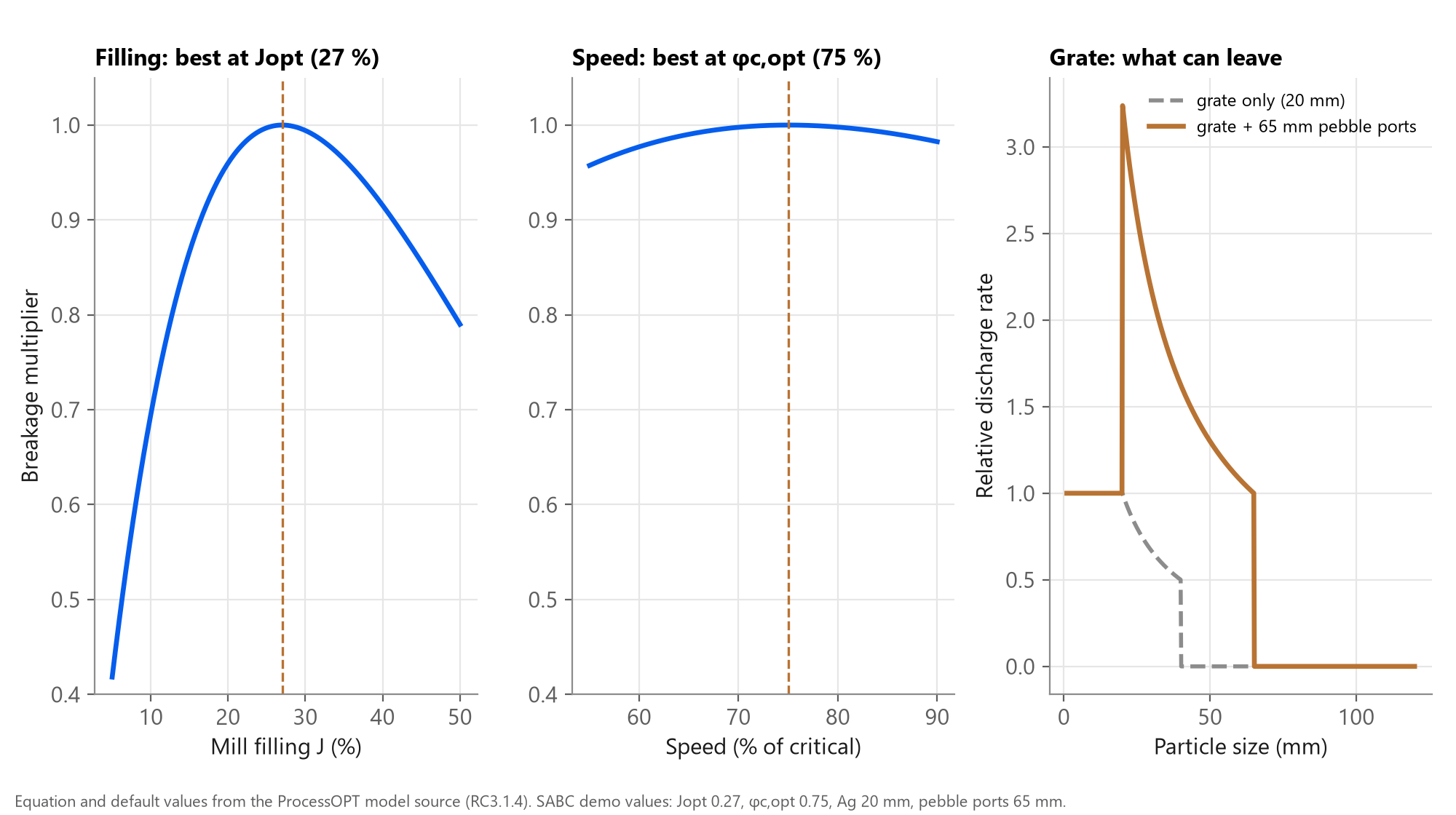
Three settings shape the response: filling, speed and grate
Note the pebble-port window: particles between the grate aperture and the port size leave faster than through the grate alone, which is why pebble ports raise pebble flow to the crusher.
2 Objective
A SAG model that tracks filling, power and product size well enough to test control before it reaches the plant.
By the end you will have
- A SAG Mill PMB node that responds to feed rate, feed size, water and speed
- Live filling J, weight, power, discharge P80 and residence time as tags
- A Morrell power cross-check you can calibrate against the motor
- An optional live feed size from the Rock Analyzer
- A model ready for the SAG expert system or MPC to run against, offline
3 Step by step
Every screen below is a real ProcessOpt screenshot.
Step 1 - Add a Simulation node and wire it into the scan
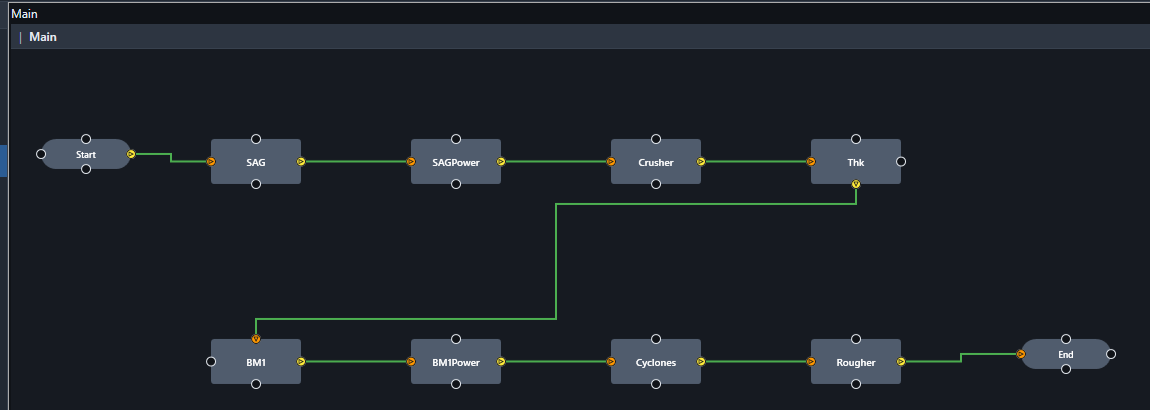
Every model in ProcessOpt runs inside a Simulation node. The node is executed once per scan cycle in the order of the graph, so place it after the logic that writes its inputs and before the logic that reads its outputs.
- Project Configuration > Logic Editor
- Right-click the canvas > add a Simulation node, name it SAG
- Connect Start > SAG > End so it runs every scan cycle (1 s here)
- One node per unit: the demo project has eight models on one canvas
Step 2 - Choose the model type and name the I/O tags
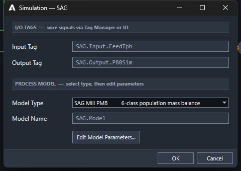
- Double-click the node to open the Simulation dialog
- Model Type: SAG Mill PMB (6-class population mass balance)
- Input Tag and Output Tag are the two headline signals; every other result gets its own tag automatically
- Press Edit Model Parameters... for the full model sheet
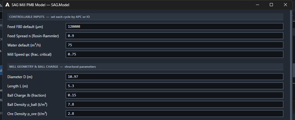
Step 3 - Controllable inputs, mill geometry and ball charge
Use the effective inside-liner diameter and the belly length. The speed and water values are only starting values: the moment a tag is wired to IO or a controller, the live value wins.
- Feed F80 120,000 µm and Rosin-Rammler spread n 0.9 build the feed size distribution
- Water 75 m³/h and speed φc 0.75 are tag defaults: APC or IO overwrites them every scan
- D 10.97 m, L 5.3 m (inside liners), ball charge Jb 0.15
- Densities: balls 7.8, ore 2.8 t/m³
Step 4 - Grate, discharge and breakage parameters
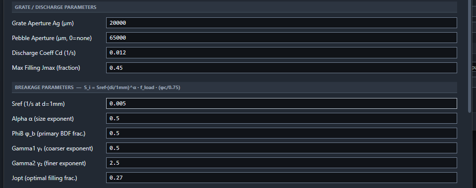
Calibration order that works on most plants: first Cd until the simulated filling J matches the bearing-pressure or load-cell estimate at the design feed; then Sref until the discharge P80 matches a survey; leave φb, γ1, γ2 at defaults unless you have drop-weight data.
- Grate aperture Ag 20 mm, pebble ports 65 mm (0 = none)
- Discharge coefficient Cd 0.012 1/s sets how fast slurry leaves
- Sref 0.005 1/s and α 0.5 set the breakage rate at 1 mm and its slope with size
- Jopt 0.27: filling where breakage peaks; φb, γ1, γ2 shape the breakage function
Step 5 - Optional: feed the live size distribution from the Rock Analyzer
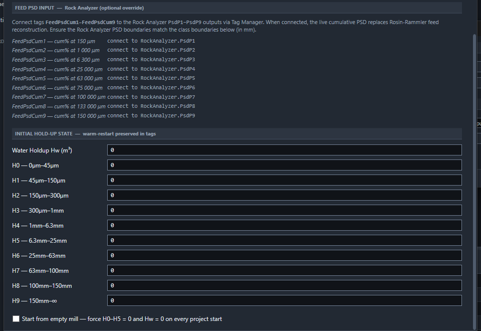
This is where the smart instrument gives the model a head start: a coarser feed shows up in the model before it shows up in mill power or weight.
- FeedPsdCum1..9 accept cumulative % passing at nine sizes (150 µm to 150 mm)
- Wire them to RockAnalyzer.PsdP1..P9 in Tag Manager
- When connected, the measured feed replaces the Rosin-Rammler estimate
- Initial hold-up H0..H9 and Hw allow a warm restart
Step 6 - Add a Morrell power node for a cross-check
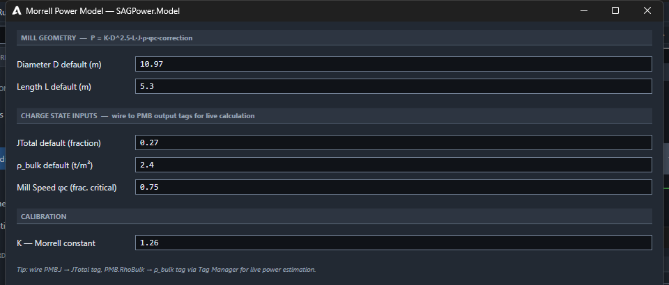
P = K·D^2.5·L·J·ρ_bulk·φc·F(φc) plus no-load power. K is the one calibration constant; start at Morrell's 1.26 and adjust by the ratio of measured to predicted net power.
- The PMB already computes SAG power with the Morrell C-model (K 1.26)
- A separate Morrell Power node (D, L, J, ρ bulk, φc) is useful to cross-check or to model mills without a PMB
- Wire SAG.J to JTotal and SAG.RhoBulk to ρ bulk in Tag Manager
- Calibrate K so model power matches the motor kW at a known load
Step 7 - Start the runtime: the mill settles at 12.4 MW, J 0.27, P80 21 mm
Runtime > Start. The SAG & Pebble page of the SABC demo shows SAG power 12,417 kW, weight 484 t, filling J 0.268 and SAG P80 20,633 µm after 30 minutes, with the screen and pebble crushers closing the loop. The SAG is a single mill, so 12.4 MW is the whole-mill power; the pebble crusher power on the same page is per crusher (the demo runs two in parallel).
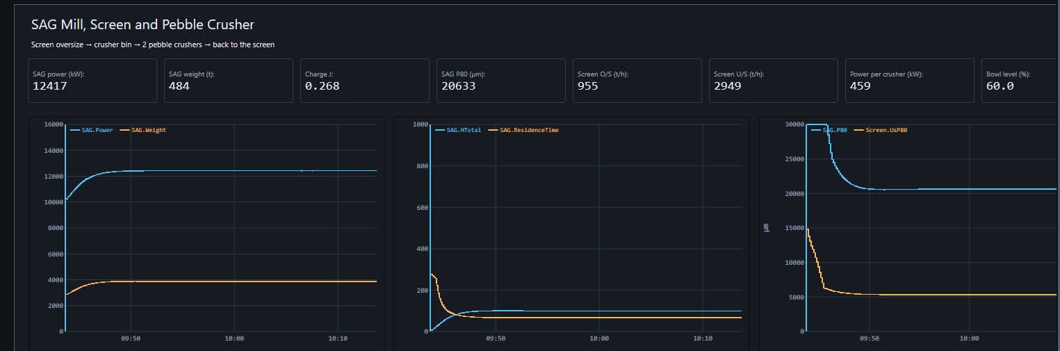
Outputs the SAG node writes each scan
| Tag | Meaning | Unit |
|---|---|---|
| SAG.J | total mill filling (balls + rock + slurry) | fraction |
| SAG.Power | Morrell C-model power | kW |
| SAG.Weight | rock + balls + water in the mill | t |
| SAG.P80 | discharge 80 % passing size | µm |
| SAG.FOut | discharge solids | t/h |
| SAG.ResidenceTime | hold-up / discharge | min |
| SAG.ToeAngle, SAG.ShoulderAngle | charge shape | rad |
| SAG.CumPsd1..9 | discharge size distribution | % passing |
Checks before you trust the model
- At design feed, J sits within 2-3 points of the plant estimate
- Model power within about 5 % of motor kW after K calibration
- P80 trend moves the right way when feed F80 coarsens
- A feed step settles in minutes, not seconds: the hold-up is real inventory
- Keep tag defaults for any input not yet wired to IO
Request a demo to build a model of your own mill with our team.
Talk to an engineerSources
- ProcessOpt RC3.1.4 - process model source code and editor dialogs, Aeterna Automation, 2026
- Mineral Comminution Circuits: Their Operation and Optimisation (JKMRC Monograph 2), Napier-Munn, Morrell, Morrison and Kojovic, JKMRC, 1996
- Power draw of wet tumbling mills and its relationship to charge dynamics, Morrell, S., Trans. IMM Section C 105, 1996
- Process Engineering of Size Reduction: Ball Milling, Austin, Klimpel and Luckie, SME-AIME, 1984
- A matrix theory of comminution machines, Whiten, W.J., Chemical Engineering Science 29, 1974
- Wills' Mineral Processing Technology, 8th edition, Wills and Finch, Butterworth-Heinemann, 2016